Introduction

Disparities between global regions have been evident in various aspects, and knowledge distribution is no exception. Wikipedia shows a significant concentration of articles tagged in Europe and North America, overshadowing contributions from less developed regions [1]. This reflects social and cultural imbalances among different geographical areas. Research by Laniado and Ribé [2] reveals that Wikipedia editors tend to focus on articles related to their cultural identity, which was further explored in [3]. Our project aims to investigate if this inequality is present in the Wikipedia excerpt [4] used in the Wikispeedia game. We want to determine if players fare better when navigating through articles related to Europe, highlighting potential geographic bias.

Geography of Wikispeedia

For our first objective, we need to classify the articles geographically, more specifically in continents. We talked before about “geotagged” articles, this information is contained in the metadata of Wikipedia articles. Unfortunately, we don’t have access to this kind of metadata. For our classification, we first automatically classified those items that in our dataset were already classified within a continent, such as countries, some geographical areas, British monarchs, or presidents of the United States. However, these articles only represented about 15% of our dataset and we wanted to classify them all since some categories such as people can be strongly related to a continent.

Luckily our beloved friend ChatGPT came to the rescue, we politely asked to classify all the articles by their name giving it only the options that were already included in our dataset for the geographic data. These options were: Africa, Antarctica, Asia, Europe, the Middle East, North America, Australia, and South America. What is more, we also gave it the category “International” as an option for those articles that were not strongly related to one single continent. As we were not considering Central America, ChatGPT considered those countries as North America while our dataset considered them as South America. In this case, we kept the dataset classification. As can be seen, the Middle East is a category because it was also a category in the initial dataset. In this case, we decided to relabel all the articles labeled as Middle East as Asia. To wrap up our classification we merged ChatGPTs with ours, classified the discrepancies manually to ensure a better outcome and we also discarded all those articles classified as International.

At this point, we are ready to go for a first naive analysis of the data. Does Wikispeedia’s excerpt have a bias towards Europe?

It seems it does, at least in terms of the number of articles, there are many more articles classified as Europe. What about the distribution of the continents among the different categories?

We can also observe a majority of European representation in most of the categories. This makes sense, if Wikipedia has more articles geotagged in Europe and North America (NA) it is not surprising that Wikispeedia does as well… but, what about NA? Well, we should always bear in mind that Wikispeedia is an excerpt of Wikipedia that is specifically targeted around the UK National Curriculum and that we discarded all International classified articles (many international contributions have been made by NA).

Main Analysis

Naive Analysis

We can make it official by now, this is an observational study. Therefore, we define a treatment and control group. The treatment group will be the paths taken by the users that have a target article classified in Europe and the control group will be those paths whose target article is not classified in Europe, in other words, the rest of the world.

Let’s dive into the paths. When a player starts a game, a start and goal article will be automatically given and the goal is to reach the article. When achieved, this is what we will call a finished path. Now, which percentage of the paths are finished and also have a start or target article that belongs to Europe? Let’s find out if there is a difference between the other continents.

Wow, that is a big difference! Almost all of the other continents have to sum up to get to the same number of paths that have a European start or target article. This makes a lot of sense, considering that Europe is the continent with the most articles.

While looking at the percentage of paths that are European and finished is quite interesting, we would also like to understand how people play and if they are more likely to be successful if the target article is from Europe. To study this, we computed a statistical t-test with the null hypothesis that the percentage of finished paths for Europe is the same as the rest of the continents.

We compute the statistical t-test between the two groups and… bingo! We get a p-value of 0.032 which is lower than 0.05. Therefore, we can say with a 5% of significance level that if a path finishes in a European target article, it is more likely to be successful.

Matching

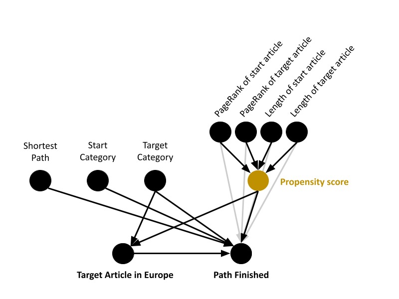
… or is it? As we have seen throughout this course, we cannot just draw conclusions over the bulk of the data, we shall perform matching. On what? Out of common sense, categories may be a good choice, one could think that it is not fair to compare a path starting from Art and ending in Music with a path that starts from Religion and ends in Science. Also, if we want to study the success rate, it is not fair to compare paths that differ in their optimal solution (shortest path). This is why we match on:

• Category of the starting article
• Category of the target article
• Shortest path

Again we ask ourselves, is it enough? As this is a fairly large dataset, we want to make sure we balance the dataset further, so we decided to compute the propensity score on some observed covariates via logistic regression. These must not be related to the way players behave because that is actually what we want to analyze, so we come up with the following:

• Length of the starting article
• Length of the target article
• PageRank of the starting article
• PageRank of the target article

To perform the matching we need a similarity function between two nodes in the graph. Based on the exercises seen in the course, we compute it as:

And we add weights equal to this similarity to the matching. In the end, the Directed Acyclic Graph (DAG) of our observational study looks like this:

Once we have defined our matching, we compute it and we check that all the confounders that we considered follow approximately the same distribution for the treating and control groups. In the following figure we will compare results before and after matching. Plots 1 and 2 correspond to the difference in the target’s and start’s category, plot 3 to the difference in the shortest path, plots 4 and 5 to the difference in the target’s and start’s PageRank and plots 6 and 7 to the difference in the target’s and start’s length.

Well… these are some strange results. First, why are the categories not the same, if we are matching on them? Our dataset contains several categories for each article, we don’t mean subcategories, we mean a whole different branch of category. For example, the article “Children’s Crusade” is categorized in History but also Religion, makes sense right?. We matched when articles shared at least one category and this is why we have slight variations. As we can see in plot 3, this doesn’t happen because there is only one unique shortest path (shortest number of steps).

As of the last two pair of plots they correspond to the propensity score matching. We must recall that the propensity score of a data point represents its probability of receiving the treatment, so we don’t expect an exact matching. We observe that in some cases the difference between the two matched groups becomes smaller.

Observational Study

Finally, we can draw some conclusions. We perform the same statistical as before, that is the null hypothesis being the percentage of finished paths for Europe is the same as the rest of the continents. Let’s see what we obtain…

There is no significance?! We get a p-value of 0.857 which is higher than 0.05. Therefore, we cannot say with a significance level of 5% that if a path finishes in a European target article it is more likely to be successful. However, we are not upset, as we always say, no results are results. After performing matching we were able to balance the dataset so the results obtained were more trustful, and they show no significance, even if before it appeared to be. This shows that what can be perceived in a well-named naive analysis is not a picture of reality but further analysis is needed.

Conclusion

Of course, we still have to take into account that our work may not be perfect, in observational studies there are observed and unobserved covariates, and their consideration (or not) can shift the results completely. One of these factors, for example, could be the participant as not all people who play Wikispeedia have the same knowledge about all categories. By not controlling this confounder, we could have two different participants with different knowledge, one in the treatment group and one in the control group. The one with more knowledge would do better and probably not because the target article is European or not.

Another unobserved covariate could be the date on which each path was played. The world changes very quickly and people are often more aware of events that happened recently. This is why a participant who played the game in 2008 can play very differently than one who played in 2012 as their focus is on different events. Our dataset contained date information, the problem is that from 2008 to 2011 only the completed paths were included, so our analysis would either be too biased or too incomplete. Therefore, we decided to not include it in the matching.

These are some examples of confounders that were not taken into account in this study but even further analysis could be done on unobserved covariates like sensitivity analysis. What we intend to say with this final comment is that we should always be skeptical about our results and not take them for granted.

References